World Building

A bit more background before these blog post start getting into the development meat.

I started coding for this project back in 2020, using C#. I tend to think fairly holistically when I’m developing a new project - which means that I develop a whole bunch of support code in library form and then slap it all together into a rough prototype to refine and test.

Luckily, in this instance, I wasn’t starting totally from scratch. Back in about 2012 I had written a bunch of game support libraries (graphics/sound/state management etc.) in C# targeting XNA/MonoGame for several game projects that got released on a few formats (Creatures & Castles, Chromatic Aberration, Zen Accumulator) for Google and Sony. It wasn’t much, but it paid the bills for a few months and kept the lights on.

Unfortunately, XNA/MonoGame had fallen out of favor, so I started the process of selecting a new backend target. I settled on Raylib.cslo, as it seems to be relatively simple, well-supported across multiple platforms and had a clean XNA-like interface.

After updating my core libraries to support the new backend, I also wrote some additional support libraries focused on procedural generation useful for a Roguelike, such as map generation, path finding, and several other variant DSLs that will be covered in later posts.

I even got a decent prototype up and running, which allowed for full procedural landscape generation in real time, using a chunk system to generate persistent chunks on demand.

Land Mass and Biome Generation

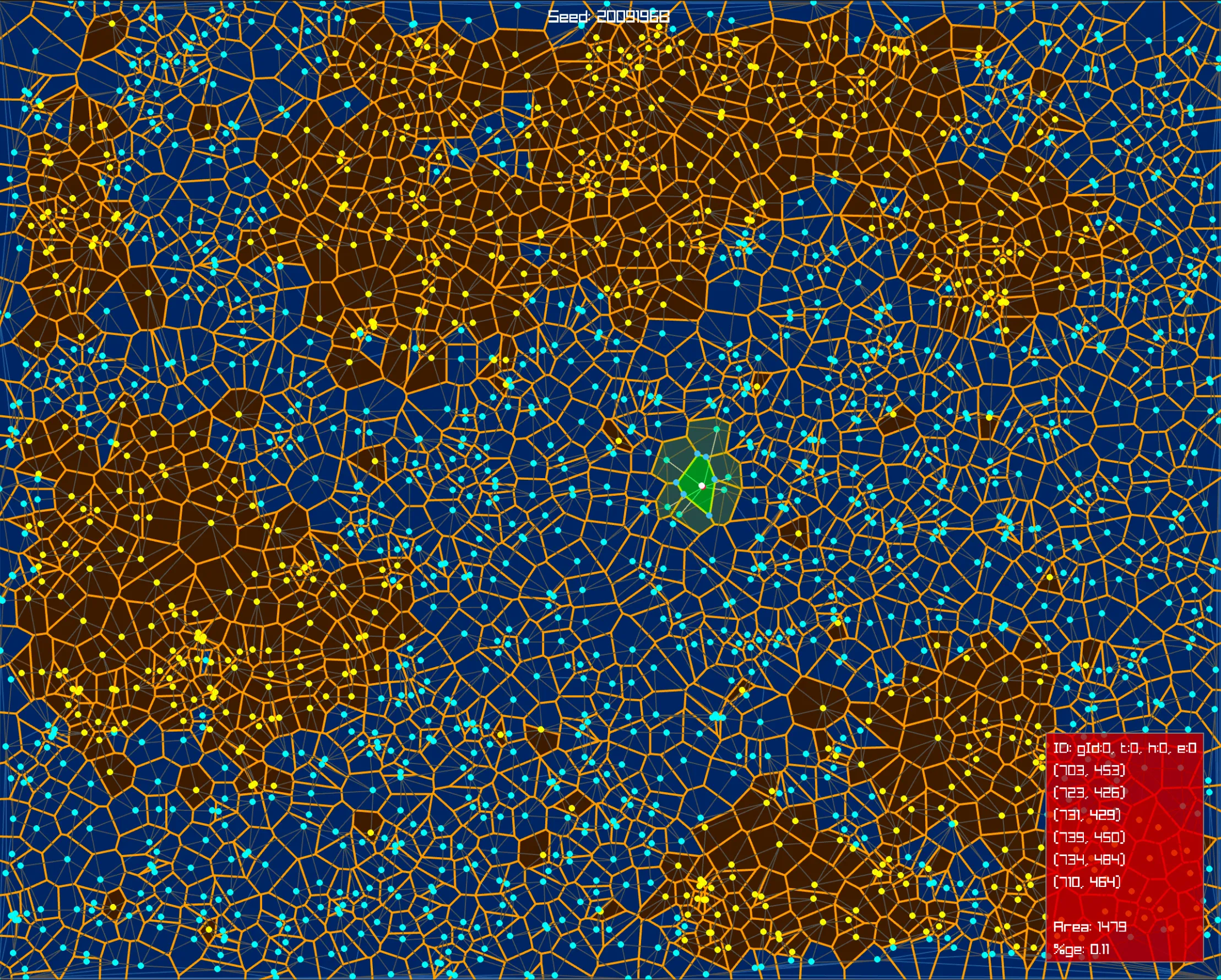
There’s nothing particularly groundbreaking about the landscape generation technique that I used here; it’s a Voronoi diagram, shown in the previous image, based on an initial seed and a number of other ancillary parameters (land/sea ratio, number of continents, number of islands etc.).

As an aside, I initially chose purely random points for the centers of each Voronoi cell, but this ended up not being optimal as shown in the previous picture, where you can see that the points are not evenly spaced, and consequently the Voronoi Cells have a significant variation in size. I then switched to using Poisson Disk generation to create the initial points which allowed for the creation of much more evenly sized Voronoi cells.

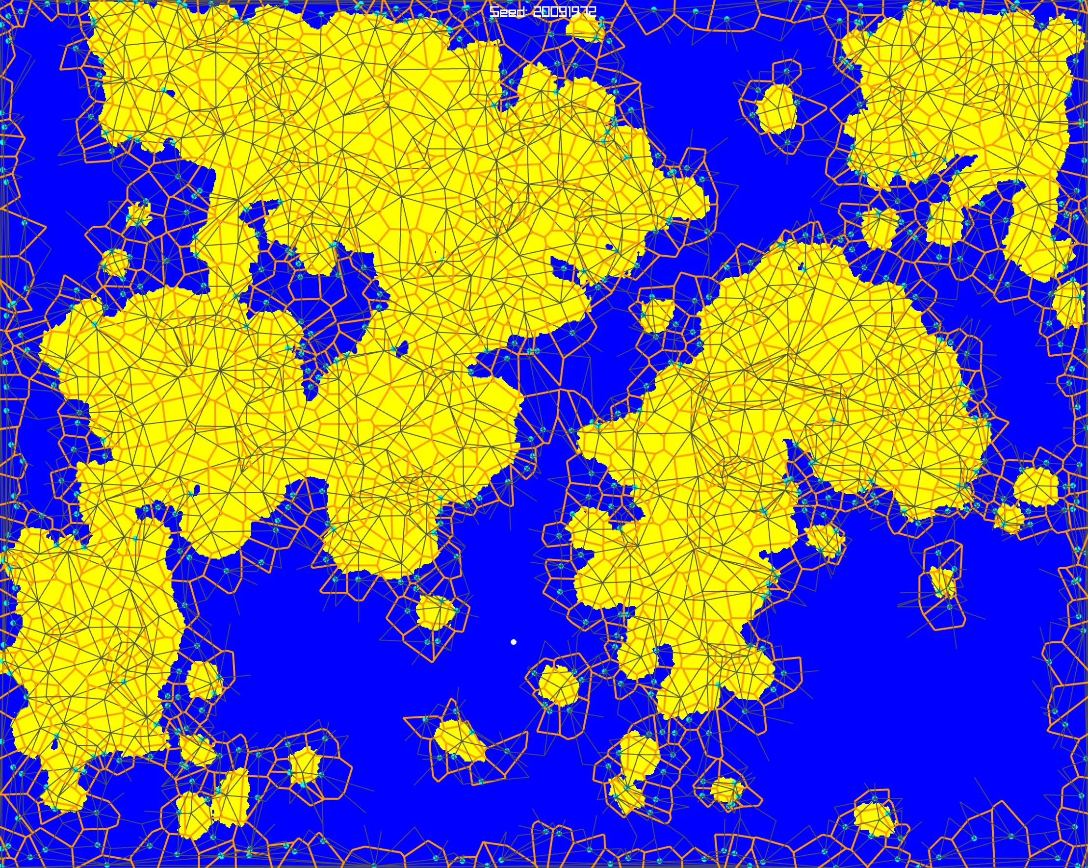
The only area where I may have innovated slightly (in that I didn’t find anyone else doing exactly the same thing), is that once I had my initial Voronoi diagram, I made heavy use of GLSL shaders to perform further processing. For example, in the next image, you can see that the edges of the land are rounded. This was simple; I used a jitter filter, followed by a blur filter, followed by a threshold filter to roughen out the straight edges of the polygons and create a more naturalistic coastline. By offloading this job to the graphics card, it made the map generation virtually instantaneous. Other worldgen packages I had looked at took a few seconds minimum to produce similar output. (Admittedly, they may have been a lot more rigorous in their worldgen simulation than I was being, but if the output is indistinguishable, why do the extra processing?) As an additional simplification step, I deleted all internal cells that were totally surrounded by sea.

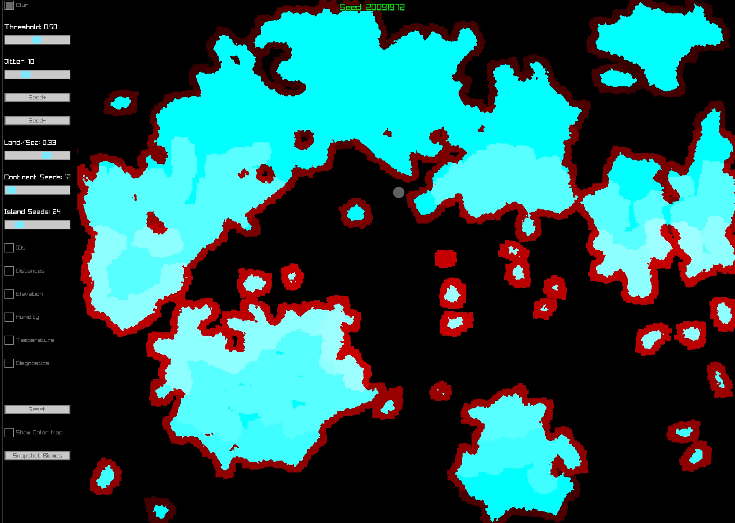
The next image shows the biome assignment, encoded as texture values. It’s a bit difficult to see because the encoding is not eye-friendly, but again, by doing this via shader allowed for extremely rapid execution time. The biomes are encoded in the red channel, which is why the landmasses show as slightly different shades of light cyan. You can also see the edges of the landmasses clearly defined with a red outline, which show the effects of the threshold slider (at the top left of the image). If that slider was reduced to zero, there would be no red outline. At maximum, there would be a much larger red outline (meaning more land erosion).

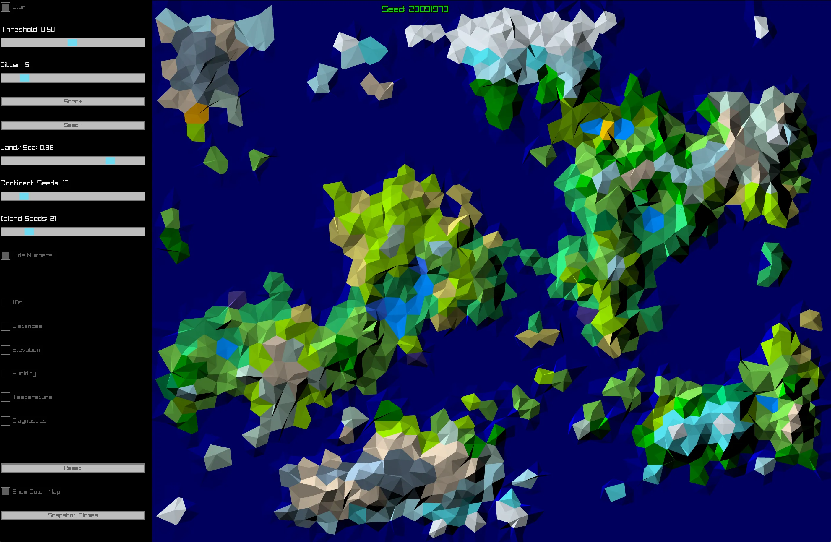
The next image shows a cleaner polygonal view of the generated biomes combined with the height map. Honestly it wasn’t much use other than for a visual sanity check, but it did look pretty, which is why I included it here.

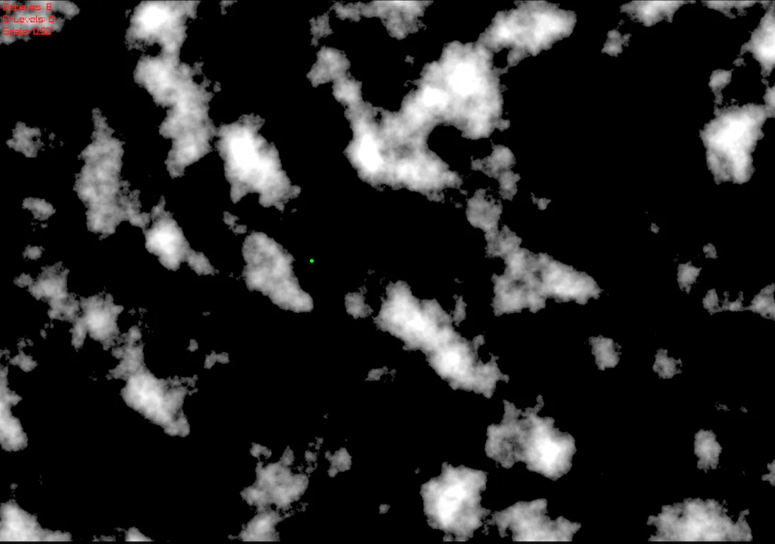
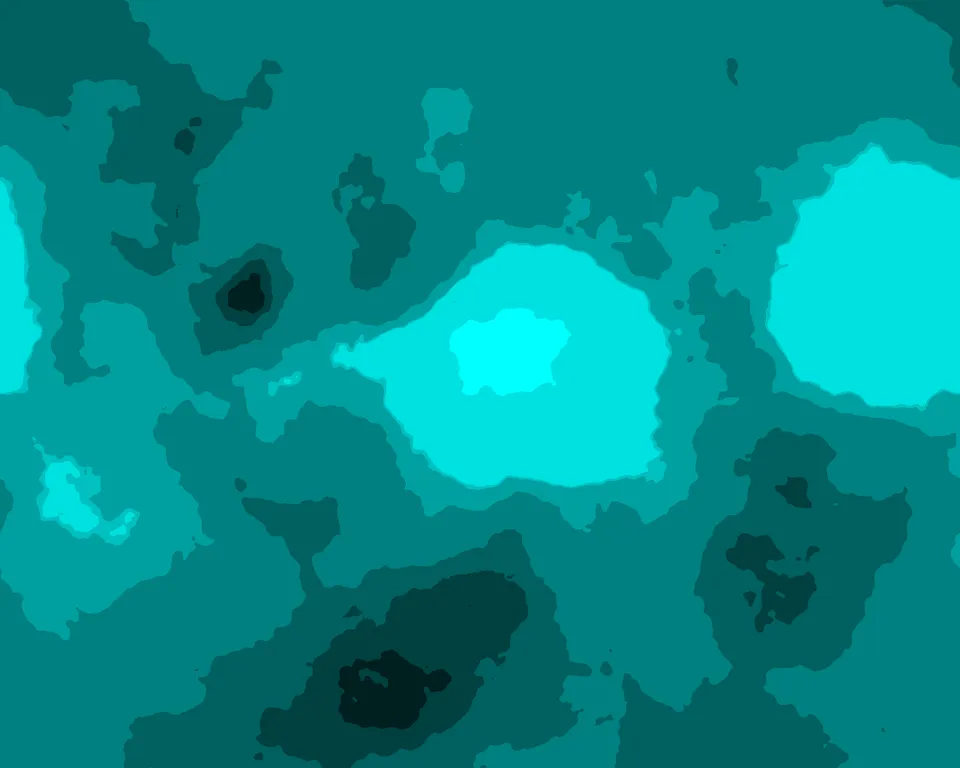
To decide what biomes went where, I used another three generated shader textures. The first two were for altitude and rainfall. The altitude map was modulated with the biome texture to ensure that land near the sea was close to sea level. Both of these used Simplex Noise as the base technique for their implementations. The third map was a temperature map. This was implemented in a simple fashion, first by creating horizontal stripes representing temperature, and then applying a seeded random vertical distortion across the texture.

The following three images show the modulated altitude, moisture and temperature maps respectively.

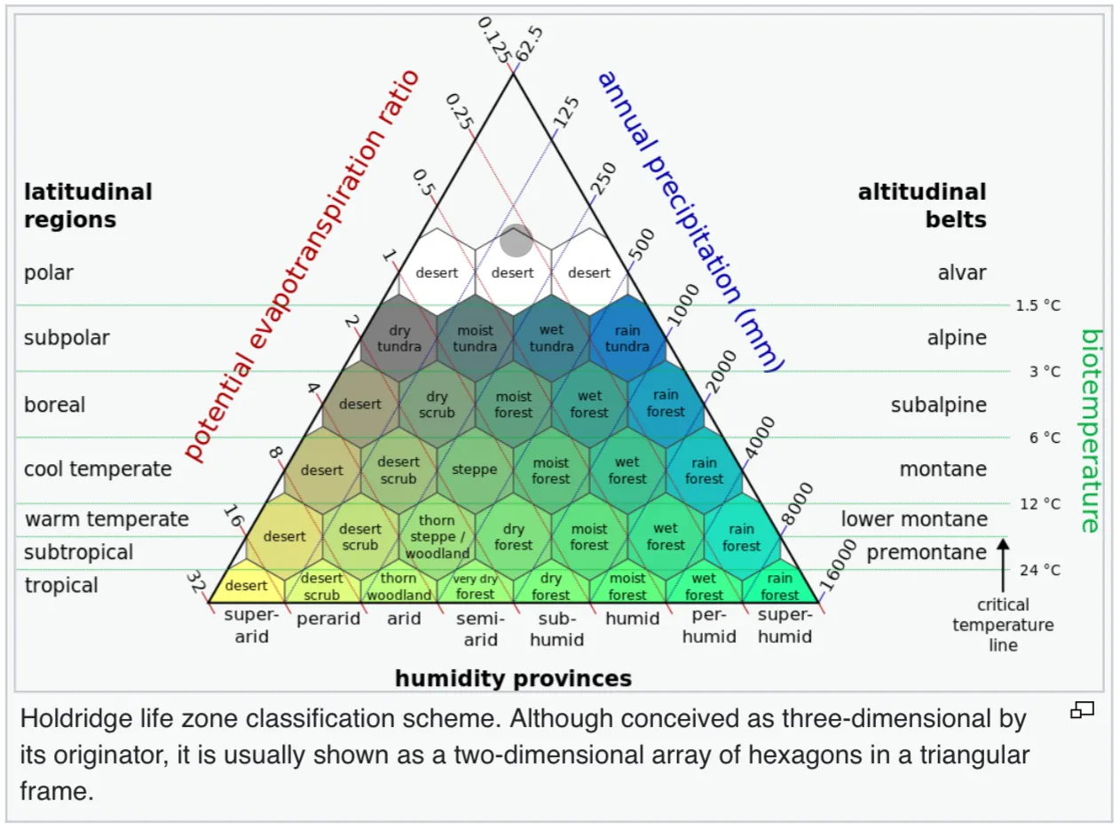
I used the three maps as a 3D lookup into a pre-defined biome table to assign biomes based on altitude, temperature and rainfall. The table itself was based on real-world biome zoning - specifically the Holdridge life zone classification scheme, shown here (sourced from Wikipedia).

The end result of this process was a large world map of biome info, comprising biome type, altitude above sea level, average temperature, and average rainfall.

Populating The World

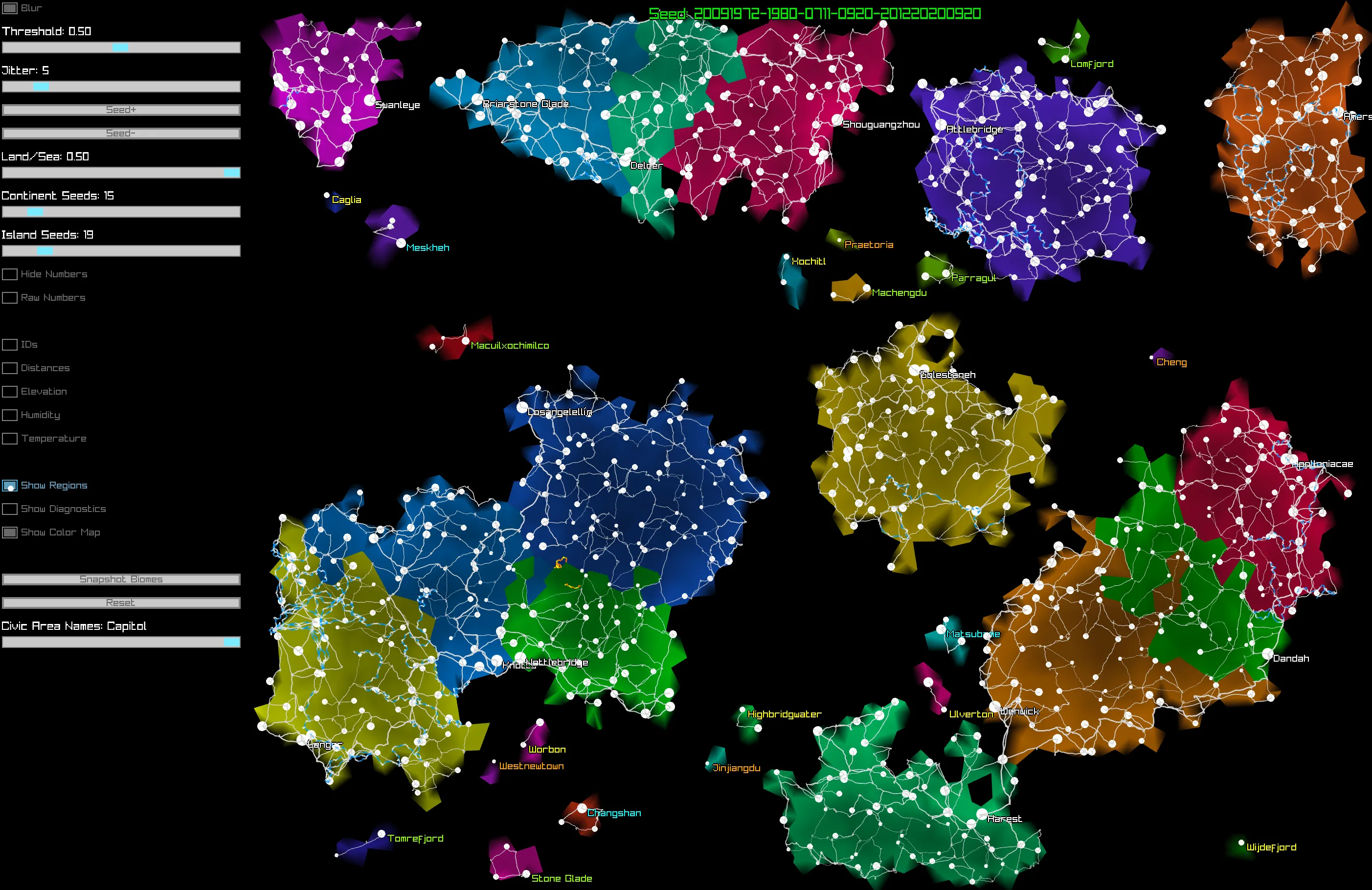
Once the biome map had been created, the next step was to divide the world into geopolitical regions. This part was actually fairly trivial due to the way the original Voronoi Graph was generated. One of the initial parameters lends itself directly to assigning such regions - “Number of Continent Seeds”. By retaining the continent number for each biome region, we can use that directly as an ID for the geopolitical region.

Once we have our geopolitical regions, we can decide where the capital city of each region goes. In order to do this, I used a fairly arbitrary set of “scoring” parameters for each Vorinoi Point. (Voronoi Points are points that define the edge vertices of each Voronoi Cell in the graph). The main reason for choosing just to evaluate the edges was for speed, even though this would result in only an approximation for best city placement. Once each region point was scored, a capital city was placed a the highest scoring point. Following that, cities, towns and villages were placed at other candidate points in order of descending score.

Each region was then randomly assigned a culture (e.g. Germanic, English, Japanese etc.) and the cities and towns were named using Markov Chains seeded with location names from that culture.

The final step (for capital cities) was to generate a road network between the capitals. Again, for simplicity and speed, the roads were routed along the edges of Voronoi Cells where possible, taking the lowest scoring route, with the score based on altitude change, terrain type (including whether there was already an existing road that could be reused), and overall distance, as well as a massive penalty for straying outside the geopolitical region. Once all the capitals had been linked, each city had roads formed for any cities or towns within a certain range, then each town to any other towns and villages, and then each village to other villages. As a final step, any unconnected settlements would be connected to the nearest road where possible.

The resulting geopolitical map ended up looking something like the image below. Note that the difference in internal shading for each color-coded region is based on the scoring for the Voronoi points within that region (normalized for the region). As can be seen, I also weighted for proximity to a coastline.

From this point, I had all the data I needed to be able to generate a top level tile based map, with a one-to-one relationship between source map pixels and biome tiles. Initially I just focused on having the landscape display correctly, producing output that looked something like the following image.

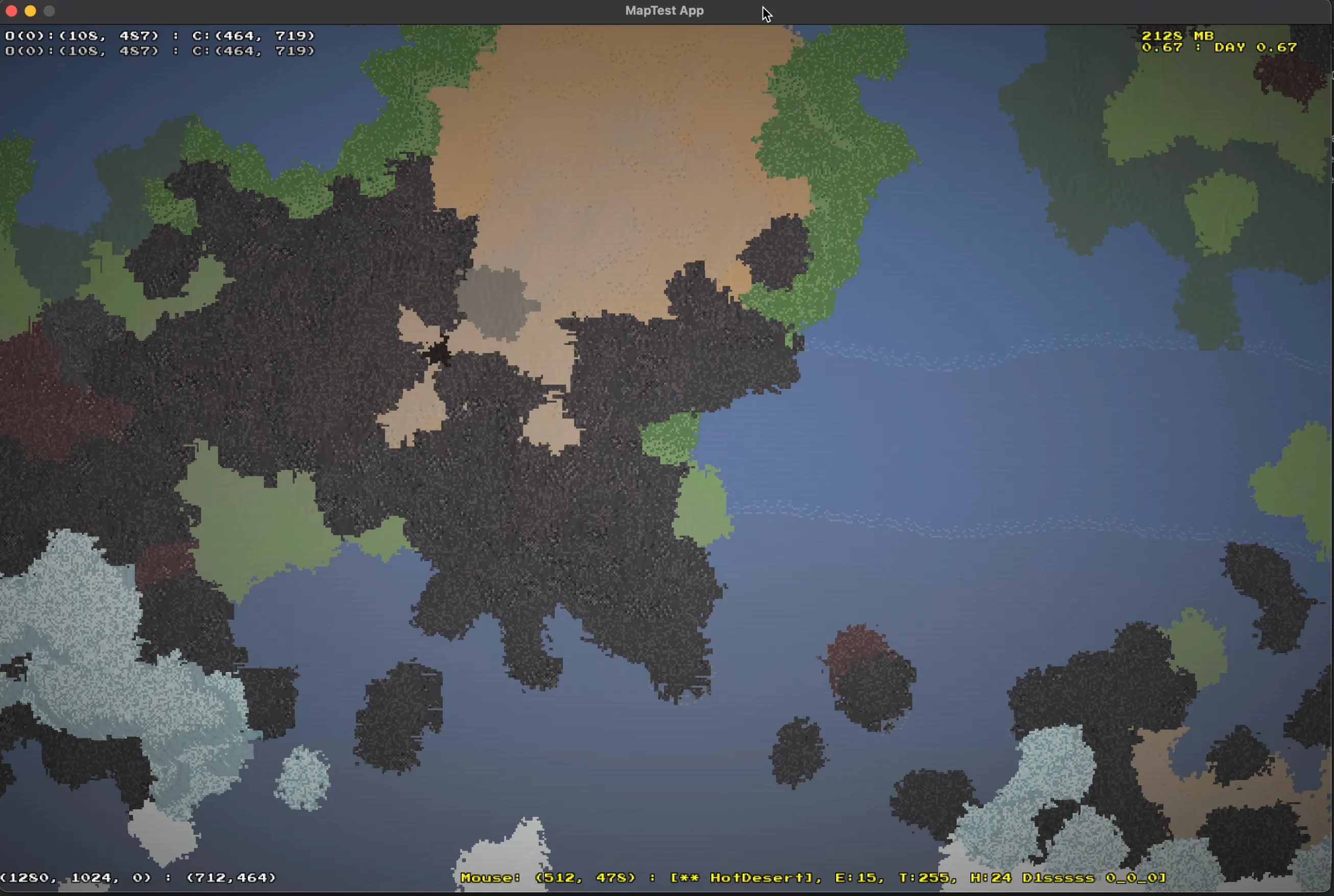
This was a good start. I now had a world that could be represented as tiles. However, it was only the size of the initial image. Clearly this wouldn’t do for a large and expansive game world, and it wouldn’t be possible to create a full tile map of the world the size I would want due to memory and performance constraints.

The solution here was to use a procedural zoom to generate more detail on demand as we zoom in on the map. The tricky part was making sure that it was internally consistent. To do this, I conceptualized the map as being a set of layers divided into rectangular chunks, with the original map (as shown previously) being layer 0 and containing exactly one chunk exactly the same size as the map. Each subsequent layer represented a 2x zoomed in version of the previous layer. That is, layer 1 would be double the dimensions of layer 0. I also realized it would be wasteful in terms of performance and storage to generate the entirety of the non-zero layers, especially as only an increasingly smaller portion of them would be visible at once. For this reason, each layer other than layer 0 was divided into small rectangular chunks of 128x64 tiles, meaning that each layer greater than layer 1 would have precisely four times as many chunks as the previous layer.

I wanted the same detail to be generated every time invariant of chunk generation ordering. In other words, if chunks A and B are adjacent, then I wanted both chunks to be generated identically no matter what order they were generated in. This proved to be quite tricky to solve, but I ended up ensuring that the zoom seed was based on chunk coordinates and the zoom level, as well as making sure that while generating, chunks only ever referred to their parent layer for tile information (and not their already generated sibling chunks in their own layer.) The zoom process then assigned tiles from top-left to bottom-right of a chunk based on a weighted random selection of possible parents tiles from the previous layer. This provided a consistent result no matter in what order chunks were generated.

For performance purposes, I kept an LRU (Least Recently Used) cache of chunks in memory, and offloaded them to disk when they fell out of the cache. Similarly, before a chunk was generated, the LRU cache and then the disk cache would be checked to see if the chunk had already been created. In this fashion, it could be guaranteed that a chunk would only ever be generated once, and consequently, any custom modifications made to that chunk subsequently would be saved.

This turned out to be quite performant, with only minimal delays for generation, caching and loading/saving. By offloading the loading/saving to a worker thread, these delays were minimized further to the point that they were barely noticeable.

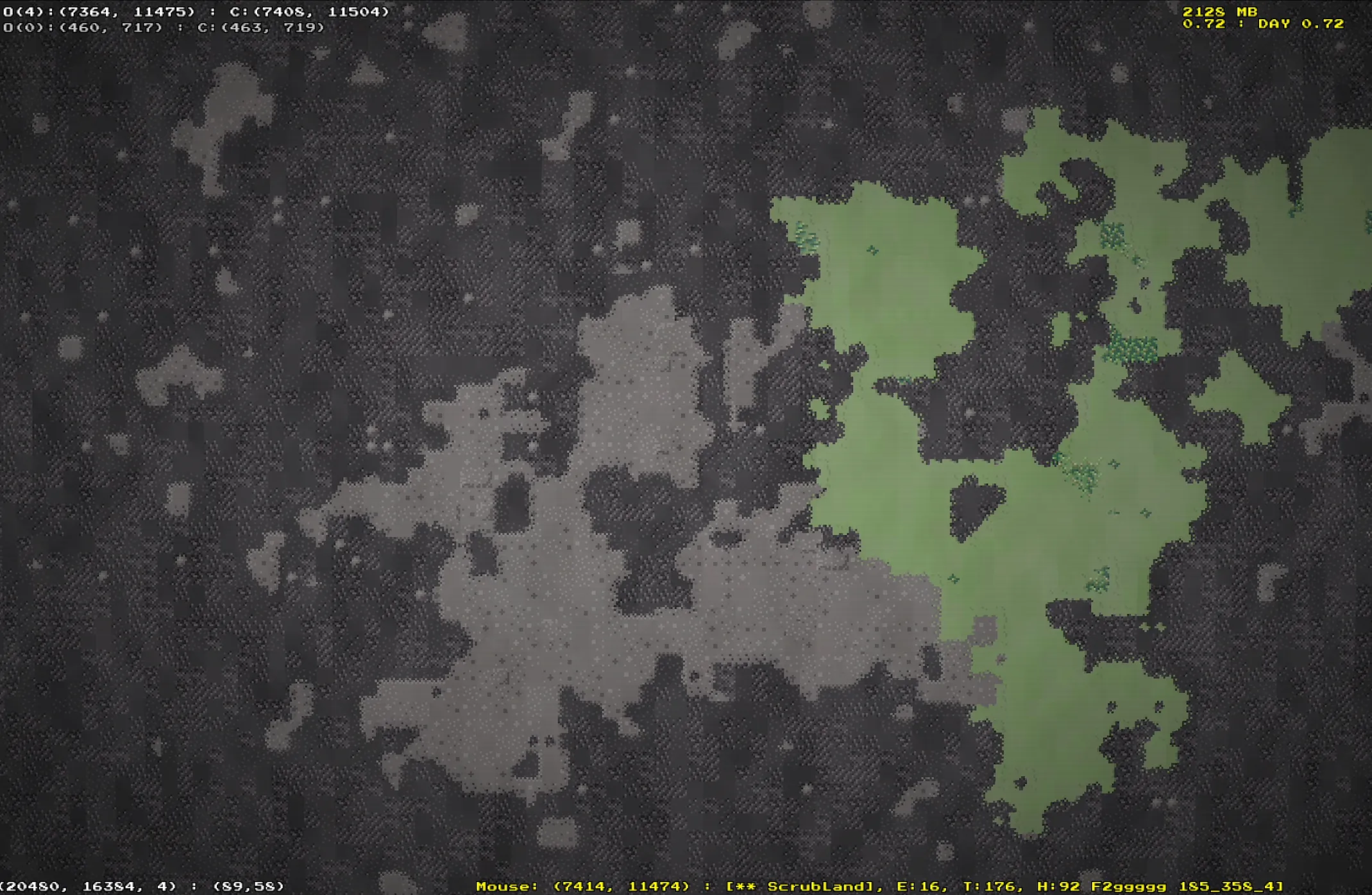
To illustrate this, here is a section of the map as generated in layer 4. Bear in mind that the original layer 0 map was 1024x768 (786432 tiles), and this layer 4 section is taken from a map zoomed by a factor of 16 (2⁴), which is 16384x12288, or about 201.3 million tiles.

If we chose to zoom to level 8, we would have a procedurally generated world with the dimensions of the original map multiplied by a factor of 2⁸, giving a final tile map size of 262144x196608, or approximately 51.5 billion tiles, roughly one third of which would be land, giving roughly 17 billion reachable tiles in the world (which, in all honesty, is probably too big to be any fun).

Realistically, a zoom level of 4 or 5 would probably be sufficient for most situations, but I have not yet decided exactly which zoom level to use. It will depend upon a lot of gameplay factors that have yet to be decided, so I will ensure that the map generation remains flexible throughout the development until a determination can be made.

Here’s a video of everything in action.

VIDEO: The proto-FAWN Engine

Now, if you read my previous post, you’ll have noticed that I talked about writing the game in Rust, so why am I talking about all of this C# stuff? I will start to cover this in my next post, but the short version is that I am taking the work I have done so far and converting it over to Rust.

There are two main reasons (and a number of smaller ones) behind this decision. The first main reason is that I wanted to learn Rust. The second reason is that I can apply the lessons learned during the development of the C# prototype to improve upon the design for the Rust conversion. Hopefully that will help offset some of the novice Rust mistakes I will inevitably make during the conversion.