Adaptive Downscaling of Pixel Art
TLDR;
Before getting started, the code discussed in this post is available here
for anyone who wants to skip these explanations and go straight to the code. PRs for corrections or improvements are always welcome.
Scaling Pixel Art
Okay, first of all, I’d like to acknowledge the scattered way my mind works. Last week I was working on a DSL for Cellular Automata, and this week I’m posting about a completely different topic. It’s not my fault — when inspiration strikes, I have to explore it. This post covers the results of those explorations.
For the game, I’m using a variety of placeholder art purchased from itch.io and other sources. Not all of it is the same scale, so even though I’ve selected graphics from different artists that fit together conceptually, there are noticeable differences in tile size. Some artwork is based on a 16×16 grid, some on 32×32, others on 48×48, and a few even on 8×8.
To make these assets look congruent, some form of scaling is required. However, due to the intricate nature of pixel art, standard scaling techniques — especially when downscaling — often introduce significant distortion, greatly reducing the quality of the artwork.
An Adaptive Downscaling Algorithm
Although there are several well-known algorithms for upscaling pixel art, I had difficulty finding automated techniques for downscaling. This isn’t too surprising, because a key feature of small-scale pixel art is the subtle shading used to imply features that aren’t actually present, leaving our brains to fill in the missing details.
I started thinking about a method to preserve this kind of detail while downscaling pixel artwork, and came up with the following methods.
- Create a scaled copy the input image using a good downscaling algorithm such as Lanczos Resampling , Bilinear Interpolation or Bicubic Interpolation .
- Take another copy of the input image and perform one or more of the following operations:
- (a) Majority Color Block Sampling
- (b) Edge-preserving Downscale
- Create a mask for the output image, to differentiate between transparent and opaque regions.
- Use the current output image, the mask, and the scaled copy from step 1 to perform a conditional replace, producing the final output image.
- Also optionally, quantize the final output to a common palette.
Majority Color Block Sampling
This straightforward technique downscales an image by examining square blocks of pixels sized according to the scale factor, then selecting the most frequent color within each block. For instance, with a 2× factor, the source image is processed in non-overlapping 2×2 blocks. It preserves transparency by making the output pixel fully transparent if the majority of the block is transparent.
The following Python code performs this operation:
def majority_color_block_sampling(img, scale_factor):
    """
    Downscale using majority-color block sampling (RGBA-aware).
    - 'scale_factor' indicates how many original pixels
      combine into one new pixel (e.g., 2 => 2x2 -> 1x1).
    - If the image is RGBA and alpha is either 0 or 255
      (fully transparent or fully opaque),
      the function preserves that transparency.
    """
    # Ensure we don't lose alpha info
    if img.mode != "RGBA":
        img = img.convert("RGBA")

    width, height = img.size
    new_width, new_height = width // scale_factor, height // scale_factor

    pixels = np.array(img)  # shape: (height, width, 4) for RGBA

    # Create an output array for RGBA
    output = np.zeros((new_height, new_width, 4), dtype=pixels.dtype)

    for y in range(new_height):
        for x in range(new_width):
            # Identify the block in the original image
            block = pixels[
                y * scale_factor : (y + 1) * scale_factor,
                x * scale_factor : (x + 1) * scale_factor
            ]
            # Flatten and handle each pixel’s RGBA
            block_2d = block.reshape(-1, 4)

            # Count transparency vs. opaque
            alpha_values = block_2d[:, 3]
            num_transparent = np.sum(alpha_values == 0)
            num_opaque = len(alpha_values) - num_transparent

            # If mostly transparent in this block => fully transparent pixel
            if num_transparent > num_opaque:
                output[y, x] = [0, 0, 0, 0]
            else:
                # Among the opaque pixels, find the most frequent RGBA
                opaque_pixels = block_2d[block_2d[:, 3] != 0]
                # If no opaque pixels exist, force transparent (edge case)
                if len(opaque_pixels) == 0:
                    output[y, x] = [0, 0, 0, 0]
                else:
                    color_counts = {}
                    for row in opaque_pixels:
                        color_tuple = tuple(row)
                        color_counts[color_tuple] = color_counts.get(color_tuple, 0) + 1

                        # simple majority
                        majority_color = max(color_counts, key=color_counts.get)
                        output[y, x] = majority_color

    return Image.fromarray(output, mode="RGBA")
Edge-preserving Downscale
This technique on its own isn’t enough, as it focuses solely on preserving edges. However, it’s useful when combined with other methods because it can highlight important details that might otherwise vanish. First, the image is converted to grayscale and run through an edge detection filter, selecting edges above a given threshold. Then, Majority Color Block Sampling is performed on the original image, and the same scale factor is applied to the edge detection data. Finally, those edges are used as a mask to retain critical details in the downscaled image.
The following Python code performs this operation:
def refined_edge_preserving_downscale(img, scale_factor, soft_edges, edge_threshold=30):
    # Ensure RGBA so we handle transparency properly
    if img.mode != "RGBA":
        img = img.convert("RGBA")

    # 1. Detect edges in grayscale
    #    We'll do this on a copy converted to RGB just for the FIND_EDGES
    edges = img.convert("RGB").filter(ImageFilter.FIND_EDGES).convert("L")
    edges_data = np.array(edges)
    edges_data = np.where(edges_data > edge_threshold, 255, 0).astype(np.uint8)
    strong_edges = Image.fromarray(edges_data, mode="L")

    # 2. Downscale while preserving color
    downscaled = majority_color_block_sampling(img, scale_factor)  # from your code

    strong_edges = strong_edges.resize(downscaled.size, Image.Resampling.BILINEAR)

    # 3. Use a mask-based approach to set only the edge areas

    # Convert the downscaled to RGBA
    color_data = downscaled.convert("RGBA")

    # Step 3a: Add partial opacity to the mask so it doesn't produce pure black
    # We'll do this by converting edges to RGBA and adjusting alpha.
    mask_rgba = Image.new("RGBA", color_data.size)
    if soft_edges:
        mask_rgba.putdata([(0, 0, 0, v) for v in strong_edges.getdata()])
    else:
        mask_rgba.putdata([(0, 0, 0, 255 if v > 0 else 0) for v in strong_edges.getdata()])
    #
    # Now each pixel has alpha = 0 or 255, matching edge map.

    # Split out the RGBA channels
    r_c, g_c, b_c, a_c = color_data.split()  # color_data is RGBA
    r_m, g_m, b_m, a_m = mask_rgba.split()  # mask_rgba is RGBA

    # Merge them so the final image has R/G/B from color_data and A from mask_rgba
    final = Image.merge("RGBA", (r_c, g_c, b_c, a_m))

    return final
Conditional Replace
During this step, the final output is produced by using the naively downscaled image (from step 1), the alpha mask (from step 2), and the image with preserved edges (from step 3). Pixels specified by the mask are conditionally replaced in the final image based on opacity thresholds, ensuring that transparent or minimally opaque areas are properly handled. This combines the smoother downscale with sharper, retained details from the edge preservation step.
The following Python code performs this operation:
def conditional_replace(
    downscaled_original_img: Image.Image,
    second_img: Image.Image,
    mask: Image.Image,
    alpha_min: int,
) -> Image.Image:
    """
    for each pixel in 'second_img' specified by the mask:
      - If second_img's alpha < 255 AND the downscaled pixel's alpha is > 0,
        replace that pixel in second_img with the downscaled pixel.
      - Otherwise, leave second_img's pixel as-is.
      - UNLESS the pixel to place has an alpha less than alpha_min,
      - in which case, set it to fully transparent.


    Returns a new RGBA Image.
    """

    w = downscaled_original_img.width
    h = downscaled_original_img.height

    # 2) Convert second_img to RGBA for consistent pixel access
    second_img = second_img.convert("RGBA")

    # 3) Ensure second_img is the SAME SIZE as the downscaled image
    if second_img.size != (w, h):
        raise ValueError(
            "second_img must match the downscaled_original_img dimensions: "
            f"{(w,h)} but got {second_img.size}"
        )

    # 4) Convert both images to NumPy arrays
    down_arr = np.array(downscaled_original_img)  # shape: (h, w, 4)
    second_arr = np.array(second_img) # shape: (h, w, 4)
    mask_arr = np.array(mask)
    # 5) Create a final array starting as a copy of the second image
    final_arr = second_arr.copy()

    # 6) For each pixel, conditionally replace
    for y in range(h):
        for x in range(w):
            m = mask_arr[y, x]
            if m == 0:
                final_arr[y, x] = [0, 0, 0, 0]
                continue
            # If alpha < 255 in second_img and alpha in downscaled is > 0
            alpha_2 = second_arr[y, x, 3]
            alpha_d = down_arr[y, x, 3]
            if alpha_2 < 255 and alpha_d > 0:
                    if max(alpha_d, alpha_2) > alpha_min:
                        # Replace the pixel
                        final_arr[y, x, :] = down_arr[y, x, :]
                    else:
                        # set it empty
                        final_arr[y, x] = [0, 0, 0, 0]

    # 7) Convert the array back to an Image and return
    return Image.fromarray(final_arr, mode="RGBA")
Example Output
I tested multiple images to refine this algorithm, including a house sprite and character sprite that are shown below.
- House
The following gallery shows the images produced at each step in the process, from input to final output. The gallery shows the process from the original image to the final result. The naive downscales lose significant detail, while the adaptive approach retains edges, shading, and transparency more effectively.
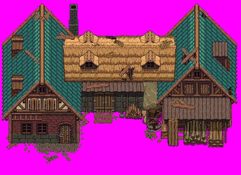

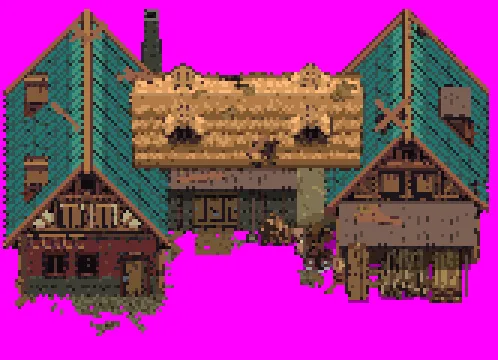
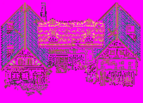
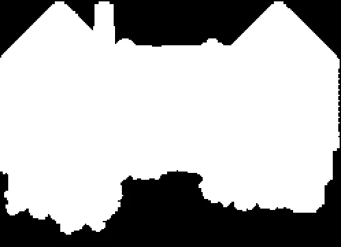
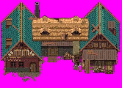
The original input image.

In the final image, scaled by 3×, minor tweaks to the edge detection threshold could yield further improvements, but it already represents a promising first iteration.

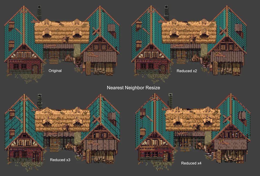
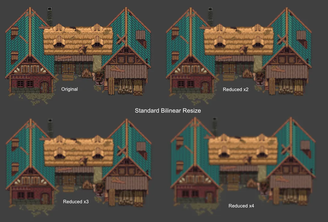
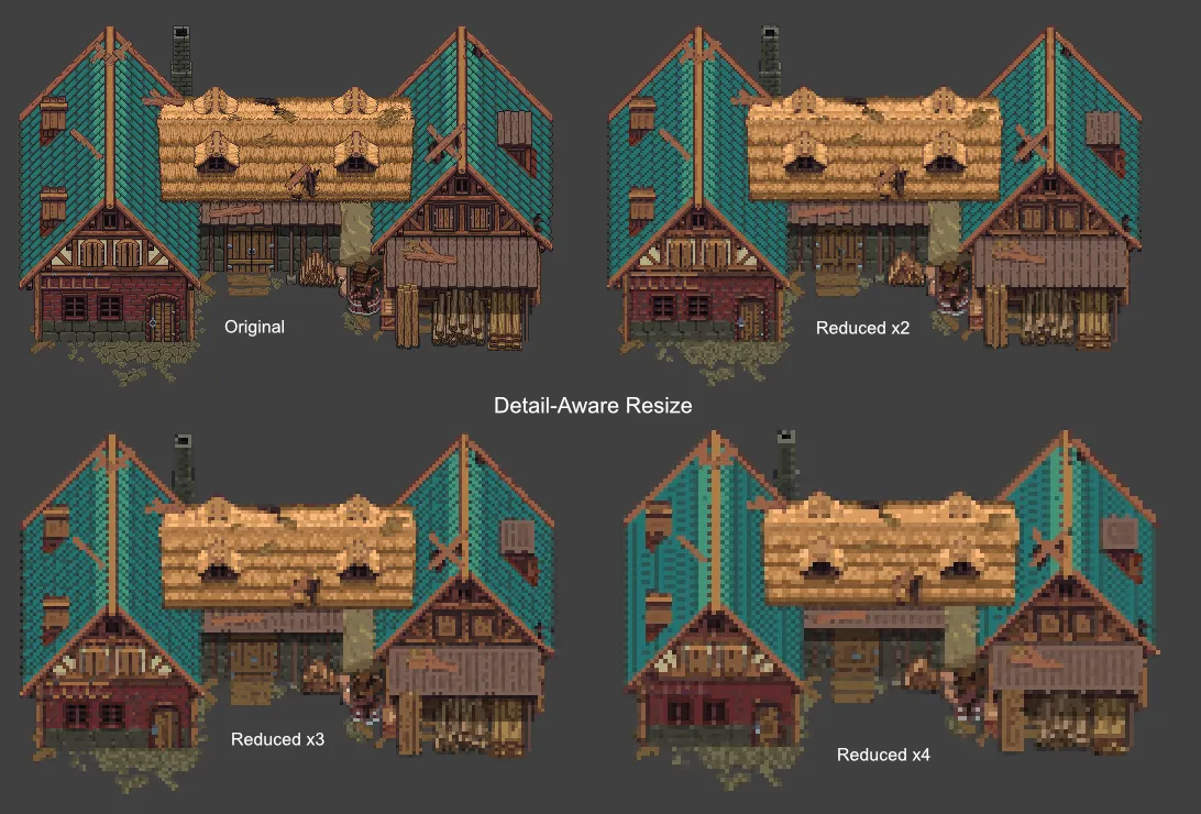
The following gallery compares downscales at 2×, 3×, and 4× using nearest-neighbor, bilinear, and this detail-aware adaptive technique. The adaptive version generally preserves shapes and edges more clearly than the others.
- Character Character graphics tend to be smaller, so the default edge-detection threshold was sometimes too sensitive — overemphasizing details like a blade swish. Even so, the downscaled results at 2× retain most of the important features, balancing smooth transitions with recognizable edges. A bonus image shows how going down by 3× is about as small as you can get while keeping enough visible detail for practical use for this example.


A final comparison of a single character frame at original size, reduced 2×, and reduced 3× highlights the difference between nearest-neighbor, bilinear, and adaptive methods, illustrating how nuanced details can be maintained at smaller scales.


Lastly, a reminder…
The code discussed in this post (plus any updates made since this post) is available here . PRs for corrections or improvements are always welcome.
Postscript
Update : I conducted additional tests of the algorithm after posting the above to assess how well it handles an “extreme” case. I chose the well-known Yoshi sprite from Super Mario World on the SNES. This was a challenging test because the sprite contains a lot of detail packed into its 32×32 pixel grid.
The following images display, in order, the input 32×32 Yoshi sprite, the 16×16 nearest neighbor downscaled sprite, the 16×16 bilinear downscaled sprite, and finally the 16×16 adaptive detail downscaled sprite.
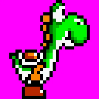

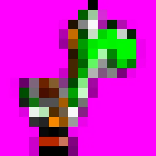
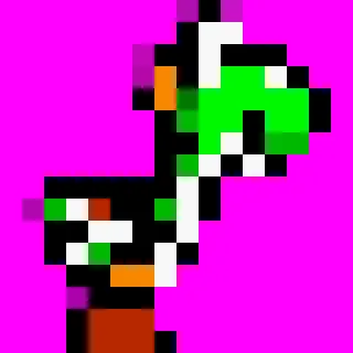
Although, in my opinion, adaptive downscaling still produces the best results, the output isn’t as good as what a skilled pixel artist could achieve. This demonstrates that with highly detailed source images, the algorithm is limited in what it can compress into a smaller space.
However, if we use the adaptive downscaling output for heavily outlined sprites as a time-saving step that can be manually tweaked during post-processing, the algorithm appears to be up to the challenge.