Machine Learning Experiments, Part 1

This post is about the first in a series of experiments to determine the utility of using an LLM (Large Language Model) to build behavior policies for NPCs. Specifically, I am setting up a simplistic gridworld environment with a narrowly defined set of rules and introducing an entity into that world in an attempt to teach it to survive.

LLMs are somewhat controversial currently for a number of reasons, both valid and otherwise. Arguments about use of others’ IP for training, energy cost of training and inference, and the threat to existing jobs being three that are examples of valid complaints. Despite that, LLMs are a powerful tool that can be used to provide content and functionality for games (and other applications) without necessarily violating the last of those complaints. The first one is a question for the lawyers and legislators, and the second is a sunk cost - inference uses very little energy in comparison to the initial training, and that’s already been done. Anyway, as a friend of mine rightfully pointed out, this post is not about the ethics of LLMs — it’s about using them to get a head start on what is otherwise a very time-consuming and often intractable problem. No jobs were harmed during the making of this post.

For a simple problem like this, the traditional approach would be to use Reinforcement Learning (RL) to develop a policy (using a technique such as Q-Learning) to iteratively calculate the best action (or range of actions selected stochastically) for the entity to take in any given state. Note that one of the key features of this type of learning is that the best action to take ONLY depends on the current state. Or, in other words, if any historical information is important to the entity, then it has to be baked into the current state. This isn’t important right now, but it will need consideration in future experiments.

Although I am starting with an very simple entity (based loosely on an ant), the overall aim of this experiment is to investigate whether LLMs will be useful in determining behavior policies for more complex game NPCs that would be otherwise difficult or impossible to train using standard RL (due to time or capacity constraints).

Question 1: Can we use LLMs to shorten the time needed to develop a satisfactory NPC policy?

Training a policy for a complex NPC from scratch would be prohibitive due to state complexity. The number of possible states for a non-trivial NPC would be huge, making policy determination an intractable problem. Traditional RL works by exploration of the state space. In other words, it tests actions (and sequences of actions) and scores the end result of a particular sequence based on a defined reward function. These reward functions are difficult to get right even in simple cases, and defining one for a complex NPC would be even harder. On top of this, RL relies on a huge number of repeated runs to iteratively search the action-state space in order to find a good policy. This is an active area of research (with a good example being the Nethack Learning Environment 🔗), and producing good results requires a lot of computing power. One of the questions that these experiments are attempting to answer is whether we can use LLMs to significantly reduce the complexity and time taken to produce a good enough policy.

Even if an LLM-produced policy isn’t ideal, it might be able to provide us with a much better starting point than a fully random policy would. We can then use traditional RL to refine the LLM-produced policy further, with the idea being that we can achieve similar results to traditional RL in a fraction of the time by short-circuiting a lot of the early learning process. (We would still have the problem of defining a suitable reward function, so that may end up being infeasible, in which case the focus should be on making sure the LLM-produced policy is sufficient.)

Question 2: Can we ensure that the LLM-produced policy is efficient for large action-state spaces?

With traditional RL, the size of the policy is a function of the number of possible actions and state variables. For a simple action-state space this size is manageable, but it can soon balloon to impractical levels with even a modest increase in either number of state variables or number of actions. This is known as the “curse of dimensionality”. The action-state space is an n-dimensional hyperspace with each action and state variable representing one axis of this space. If you have p actions and m states, adding a single new action increases the total number of action-state pairs from p×m to (p+1)×m, resulting in an increase of m additional pairs. Conversely, adding a new state variable with k possible values increases the number of states to k×m, leading to an exponential expansion of the state space.

There are various techniques to reduce the dimensionality of the state space, such as feature reduction methods that project features into a lower-dimensional space without significant loss of fidelity. However, a drawback is that these techniques require sufficient and representative data to identify which dimensions capture the most important information. In the early stages of our experiment, without enough data or an established policy, it’s challenging to determine which features can be safely reduced without losing critical information.

Even with a good policy, it’s still entirely possible that any reasonably complex NPC’s policy will be impractically large. The go-to method for dealing with this is to take advantage of the function approximation capabilities of neural networks and use a technique known as Deep Q-Learning, where the policy, instead of being represented as n-dimensional lookup table, the policy is stored in a neural network that is trained to approximate the output of the lookup table.

This approach has merit, and would likely solve the problem, but I think I’d like to try something a little simpler first, based on an older technique: Fuzzy Logic. After we have generated a policy (by whatever means) we can examine that policy dimension-by-dimension, and use a Monte-Carlo style search such as Simulated Annealing (or even a Fuzzy Clustering method) to fit the data points to fuzzy groups. If we can accurately represent the data with a few fuzzy groups per axis, this will greatly reduce the size of the policy table. We could then go on to perform other methods of dimensionality reduction if desired.

However, this still leaves us with a chicken-and-egg problem: how do we get a reasonable policy to start with? Which takes us neatly back to question 1.

Experiment 1

The aim of this first experiment is to establish a baseline and ensure that the approach is even feasible. For this experiment, we will take our simple ant-like entity and place it in a small grid world, containing a refuge, water sources, and food sources.

At any time, the entity (or should I say “ANTity”?) will have four available actions to choose from: FORAGE, EAT, DRINK and REST.

• FORAGE will cause the entity to search its immediate vicinity (defined as the entity’s current square and eight adjacent squares) for food, with a small percentage chance of food or water being revealed in one of the squares.

• EAT will cause the entity to consume food from its immediate vicinity if any is available.

• DRINK will cause the entity to consume water from its immediate vicinity if any is available.

• REST will cause the entity to regain a small amount of energy per turn if it is currently in the refuge.

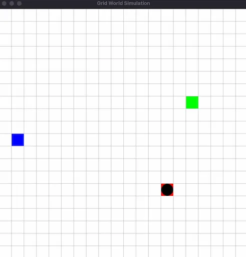
The gridworld for this experiment is a simple 20×20 grid, identical to the image. This shows a 20×20 grid with one green square (food), one blue square (water), one red square (refuge) and a black circle (entity) within the refuge.

For the initial starting conditions, the entity starts out at the refuge with the attributes 100 energy e, 100 food f and 100 water w.

Additionally, at any given time, the entity knows if food and water are present, and if so, it knows the direction and Manhattan distance to reach it, as well as the direction and Manhattan distance to the refuge.

As such, our state space comprises the following variables: Energy e, Food f, Water w, Distance to food d(f), Distance to water d(w), and Distance to refuge d(r), making our state space six dimensional (a relatively low number).

So, each “turn” we evaluate the current state of the entity, expressed as [e, f, w, d(f), d(w), d(r)], and look up the best possible action to take based on the current state values. For a simple, deterministic policy, that would be it, but in our case we are using a stochastic policy. This returns us a probability for each action to be taken in a particular state. Deterministic policies are simpler (both in calculation and implementation) but are also boring for a game - we want a bit of variability. Even though our NPCs are automatons, we don’t want them to seem that way. So, the final step is to randomly select an action weighted based on the returned probabilities, and then update the state based on the results of performing the selected action.

Once we’ve done that, we evaluate the new state and repeat the lookup, over and over until the end condition is met, which in this case is entity death.

The following table shows the effects for each action.

In addition to the effects in the table, f, w and e each decrease by 1 per turn. If either of f or w is already at zero, the loss is instead applied to e, meaning that if the entity is hungry and thirsty, e will decrease by 3 units per turn.

When e reaches 0, the entity dies and the run is over.

Note that these cost and effect values aren’t exact, as I did a lot of tweaking during the experiment, and that included the costs and effects. However, these values are not far off the eventual final values.

As the entity performs actions, these attributes are increased or decreased depending on the action and its results. After each run (i.e. when it dies) the entity is rewarded based on how long it managed to survive. This reward is then applied to each state the entity found itself in, increasing the likelihood that an action is chosen again in a specific state if the survival time was longer than the expected value (this is the survival time of the entity if it remained in the open taking no actions), or decreasing it if the survival time is less than the expected value. The delta applied to the action-state selection is the difference between the expected value and the actual value, multiplied by , the learning rate. The learning rate is a small valued constant that ensures updates to the policy are gradual, helping to avoid overshooting optimal values on the policy’s hypersurface.

This is nothing new. In fact, this is more or less standard RL (with a few minor tweaks for simplicity). The difference is our starting point — how we create the initial policy for refinement.

In order to generate a good starting policy, we can make use of an LLM as a generalized function approximator. To do this, we provide the LLM with the gridworld environment rules and constraints discussed above, and then present it with a specific state and ask it what action the entity should take in that state in order to best ensure its continued survival. In order to prevent past context affecting the action selection, we have to ensure that the LLM query is initialized with a fresh context for every query. Additionally, to mitigate the effect of LLM hallucinations, we can query the LLM multiple times for a given state and use the returned action distribution as our initial probability distribution. Note that in the future, I may experiment with asking the LLM to rank and score each available action in order to save time and hopefully improve accuracy of the initial policy, as well as query a selection of different LLMs, but given the simple nature of self-hosted LLMs, I chose not to do this for the initial experiment.

I’m deliberately glossing over how the rules and current state are presented to the LLM. There are two reasons for this. The first is that I haven’t fully evaluated the efficacy of the current method, and the second is that I think that topic deserves a blog post of its own.

There are various potential methods of sampling the action-state space, but I chose a relatively simple adaptive approach for this first test.

Firstly, I restrict all possible state variable values to integers. Then, I generate a set of coordinates for each of the six axes that encompass the corners and midpoints of each edge of the hypercube. Once these points are evaluated, adjacent selected points are compared. If those points do not resolve to the same action (within a certain tolerance level due to the stochasticity), then that axis is subdivided in two, and the new point is added to the list to be processed. This continues until an axis can be divided no further (due to the integer constraint on state variable values) or adjacent points have the same resolved action. Clearly this is not a foolproof approach, but it can get us started.

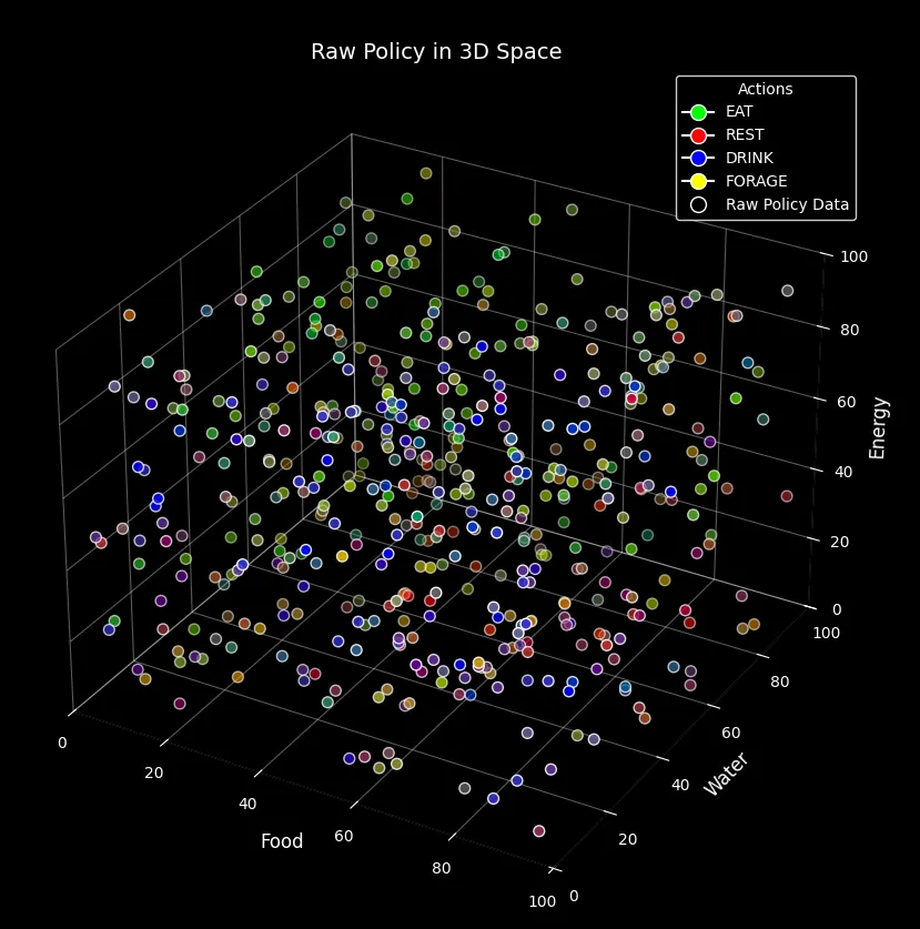
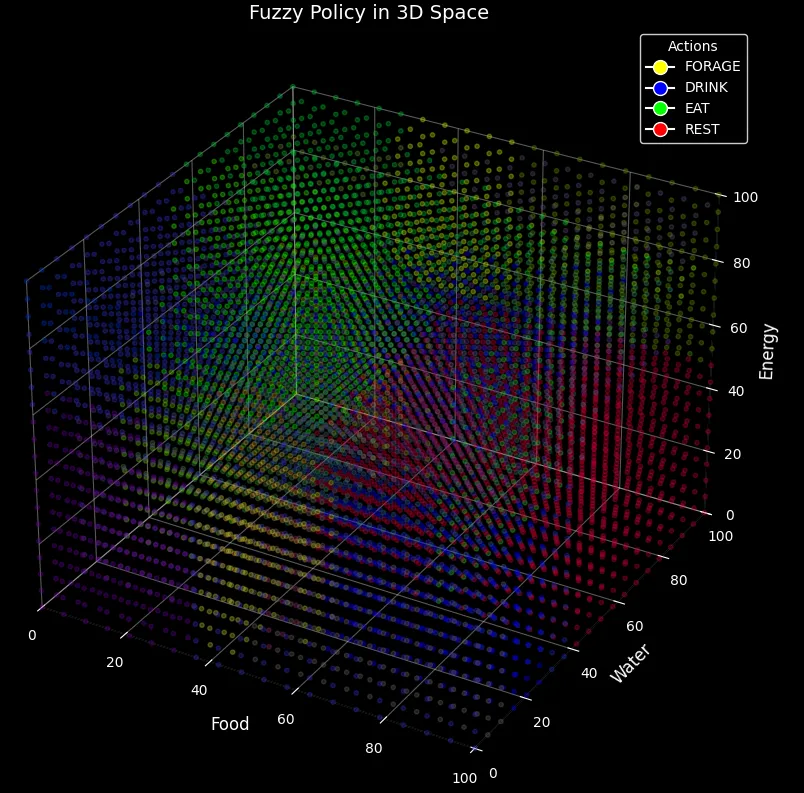
Below is a visualization of a policy generated in such a fashion. Bear in mind that while it may look pretty, it’s not actually very informative, due to having to collapse a six dimensional state space into a simulated three dimensional plot. However, what can be (just about) seen is that there are several regions of similar actions and relatively smooth transitions between them.

This makes sense from an intuitive point of view. We would not expect the best action to vary wildly between similar states. We would expect the difference between the entity having an f value of 10 or an f value of 11 to be minor; it’s still hungry and needs to EAT, assuming that other attributes aren’t in more pressing need of attention.

Now, this intuitive observation, coupled with the realization that for any non-trivial entity the policy table could get very large, lends itself to the possibility of significant optimization of storage without significant loss of fidelity. There are several possible approaches to this, but a relatively simple approach that I’m personally fond of is a fuzzy patch representation.

CONTENT WARNING: EXCESSIVE FUZZY DETAILS — CLICK TO SHOW AT YOUR OWN RISK!

What is a Fuzzy Patch representation?

A fuzzy patch representation is a method used to approximate a function or policy over a continuous, high-dimensional state space by partitioning it into overlapping fuzzy regions, known as patches. Instead of dealing with an impractically large number of precise states, fuzzy patches allow us to represent the state space with a finite set of fuzzy sets along each axis. Each fuzzy patch is characterized by membership functions that define the degree to which a particular state belongs to that patch.

Key Components:

1. Fuzzy Sets on Each Axis: For every axis (state variable), we define fuzzy sets with associated membership functions (e.g., Low, Medium, High).
2. Membership Functions: These functions assign a membership degree between 0 and 1 to any value along the axis, indicating how much that value belongs to the fuzzy set.
3. Combination of Axes: By calculating the fuzzy membership for each axis independently, we combine them to form multi-dimensional fuzzy patches that cover the entire state space.
4. Policy Approximation: The policy is then defined over these fuzzy patches, reducing the complexity of the policy table and enabling smoother transitions between actions.

Worked Example:

Imagine controlling the temperature of a room:

• State Variable: Temperature (in degrees Celsius).
• Fuzzy Sets: Cold, Ideal, Hot.
• Membership Functions:
• Cold: High membership for lower temperatures, decreasing as temperature rises.
• Ideal: Peak membership around the desired temperature range.
• Hot: Low membership at lower temperatures, increasing as it gets hotter.
• Policy: Adjust heating or cooling based on the fuzzy membership degrees.

The membership function definitions are shown in the following table:

Fuzzy Set	Membership Function
Cold
Ideal
Hot

These membership functions can be visualized as in the following plot:

Let’s consider a temperature of 18°C and calculate our membership degrees.

• Cold: Since
  :

• Ideal: Since
  :

• Hot: Since
  :

To interpret this, we can say that at 18°C, the temperature is:

• Partially Cold: Membership degree of 0.4.
• Slightly Ideal: Membership degree of approximately 0.333.
• Not Hot: Membership degree of 0.

We can also reverse the process to obtain a concrete temperature from a set of fuzzy membership values, and this is the approach we will use to optimize our policy.

Although this example is 1D, the following plot shows a 2D example and, although we can’t visualize it without a large helping of strong hallucinogenics, we can imagine how the process could be extended to an arbitrary number of dimensions.

Note also that in these examples, we are using triangular membership functions for simplicity. However we are in no way restricted to this kind of membership function. We can use any arbitrary membership function that best suits our needs.

Rather than use fixed membership sets, I instead estimate an initial number of fuzzy sets per axis based on variance, and then use a genetic algorithm to tweak the membership function parameters to find the best fit for the raw data, using cross-entropy loss as the fitness function.

The resulting fuzzy policy for the previous raw policy is shown below:

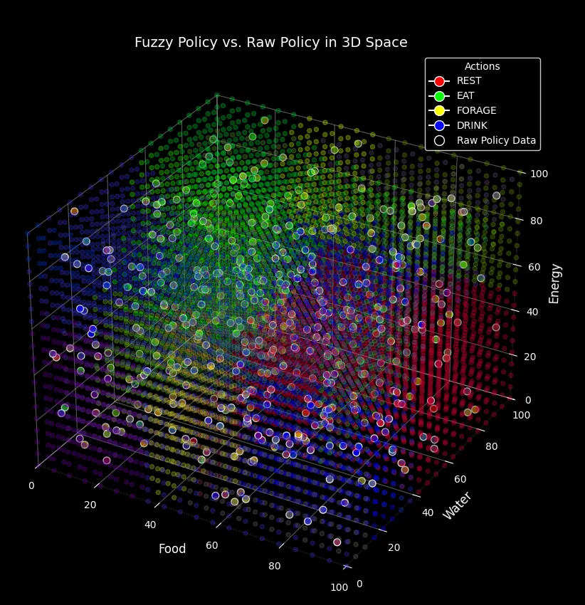
And the following plot shows the fuzzy policy overlaid onto the raw policy. Visually, it can be seen that both policies align quite well. In this particular case, the match was about 90% (obtained by comparing each populated raw policy value with its fuzzy counterpart. The fuzzy policy also required significantly less storage space, but I believe that there is still room for improvement in terms of both storage and accuracy — particularly with more complex entities.

That’s quite a lot of writing for one post, and I think that this is a good stopping point. In the next post on this topic, I will discuss the results of running the policy, comparisons between the raw policy and the fuzzy approximation, various other approaches I have taken in producing, evaluating and improving the policy, and provide more information on methods of prompt design for the LLM.